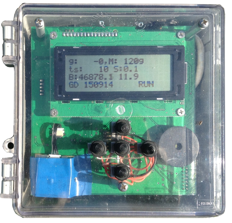
 Here we provide the results of 5 different tests that have performed as a benchmark of the capabilities of our PPM. The following test results were generated by one of our first users with the old MarkII system.The sensor is carried at around 40cm over ground and it is worth noting that a lot has changed with our PPM since these tests were performed. For example, the Mark VII features autotuning, built-in bluetooth and more sophisticated filtering algorithms which makes it superior to the Mark II demoed here.
The effects of the presence of an object made of magnetic material upon the local earth magnetic field is ruled by well-known physical laws and are independent from the type of magnetometer instrument used to make the surveys. Every such objects act much like a magnet with two poles (dipole) where one pole re-enforces the total earth field and the other pole decreases it (e.g. a cannon made of iron). Sometimes, a dipole has its two poles so much distant from each other that the survey instrument just measures the effect of the closer pole, this is then called a ‘monopole’. This is the case if a long object is buried vertically. In that case, the instrument will only see the effects of the top end. This is also the case if the object is round (e.g. a cannon ball).
To make things simpler, there are thus two main cases to consider:
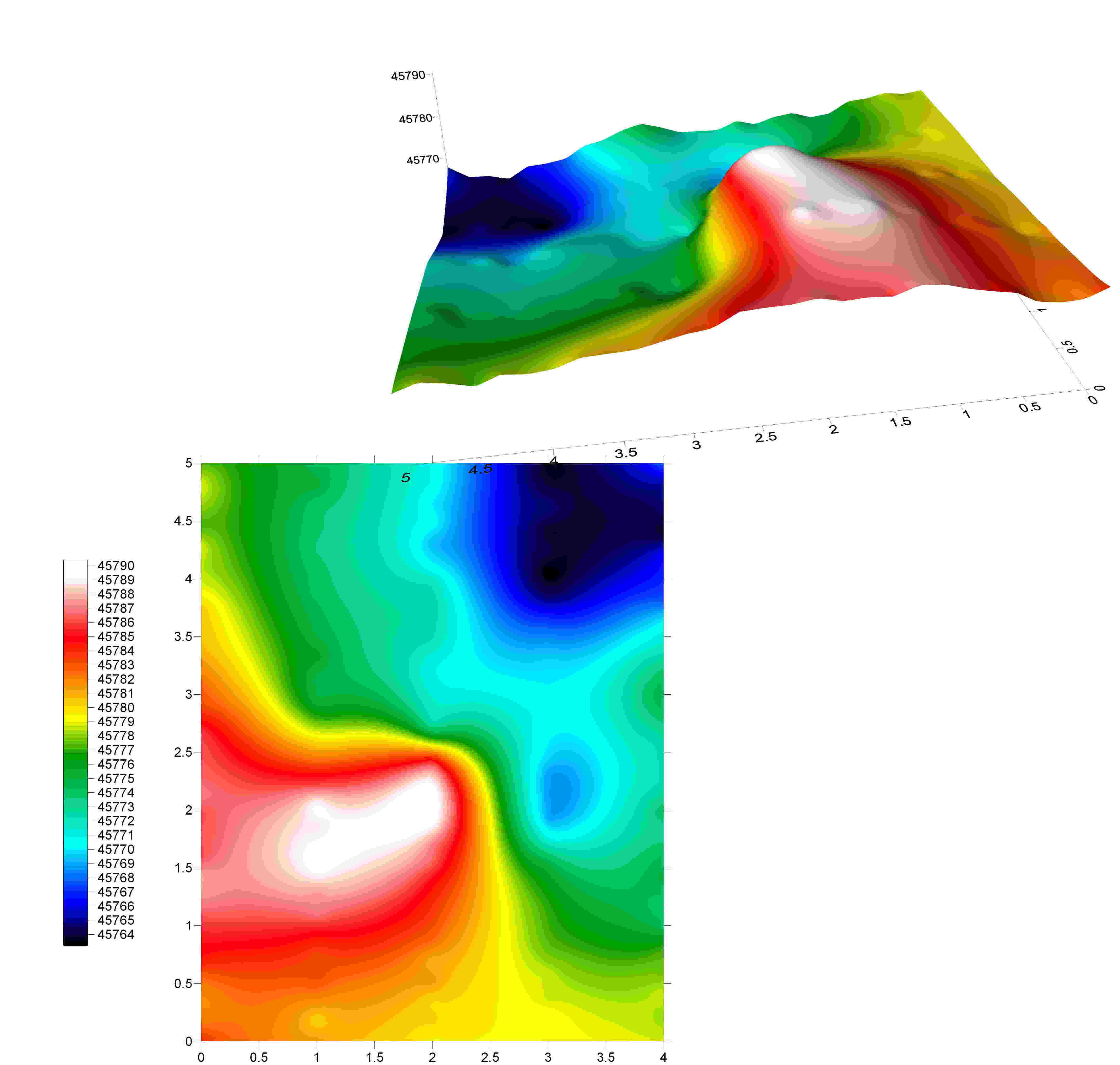
1. A monopole signature will show as a single point on the plot with a large positive (or negative) field gradient (a mountain or a valley). In that case, the object is located right at the top of the positive (or negative) peak. For an example, see test 1 which is a ball-shaped object made of the accumulation of magnetic coins. It is located at around 4,3. (Note that all the following plots are displayed with a scale expressed in meters and they were produced using our post-processing program ‘PPMUtility’ and displayed using SURFER)
2. More usually, you will see dipole signatures where you see a positive field gradient (a mountain) close to a negative field gradient (a valley). This is the effects of re-enforcement and weakening of the total earth field at the two ends of the dipole. You draw a straight line between the two peaks and the object is located just in between with its orientation given by the straight line. This is the case for all the other tests. The depth of an object can be evaluated by the sharpness of the peaks. Shallow objects generate sharp peaks while deep objects generate low and wide peaks.
If you want to fully understand the theory behind the magnetic survey interpretation rules, you should read the following document: ampm-opt in the chapter V Interpretation.
In the first test, we buried a bag of 2350 eurocent (1, 2, & 5) coins at a depth of 1.15m. The total weight of the bag was 7.7kg. The monopole signature is strong and easily detectable by our PPM.
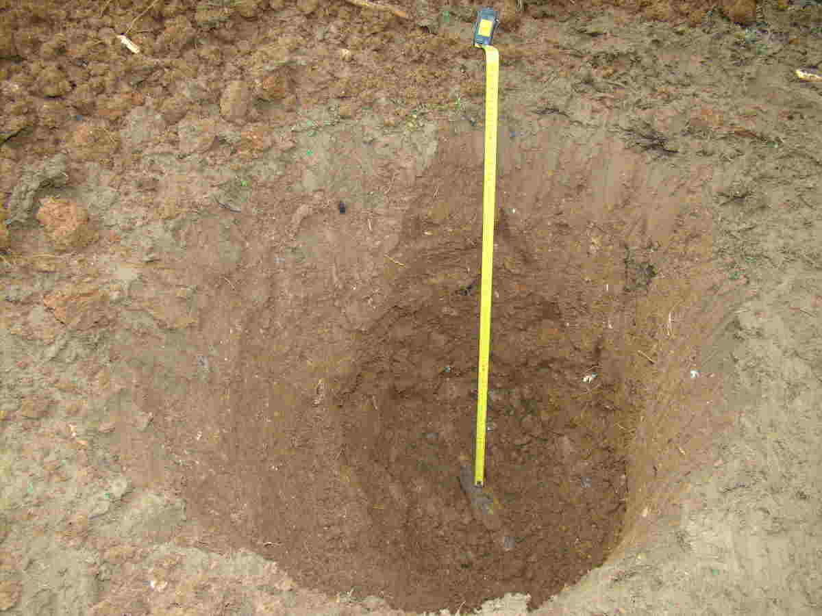
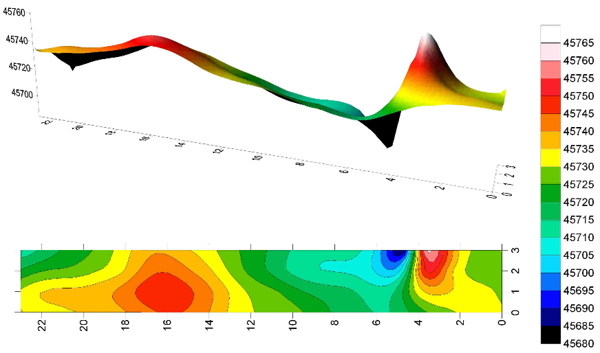
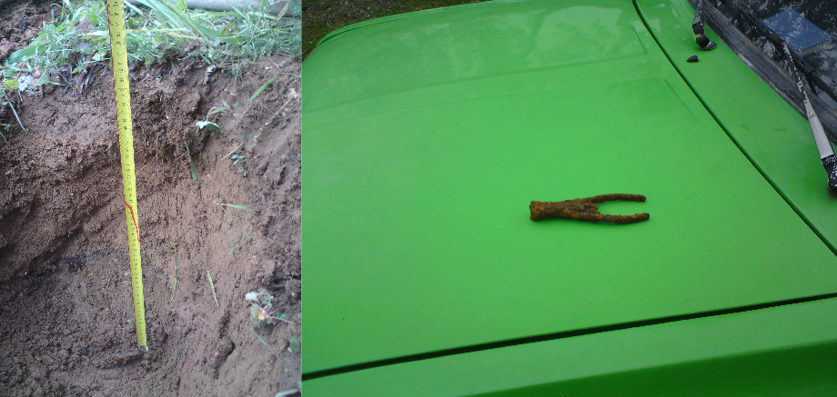 During a supplementary survey at the coins site (test 1), a high and narrow double peak (red+blue) with a magnitude of about 60nT was detected indicating an unknown dipole target. After digging 50cm deep, exactly between the two peaks, this old rusted tweezers was removed from the hole. The wide and low single red peak is the signature of the bunch of coins.
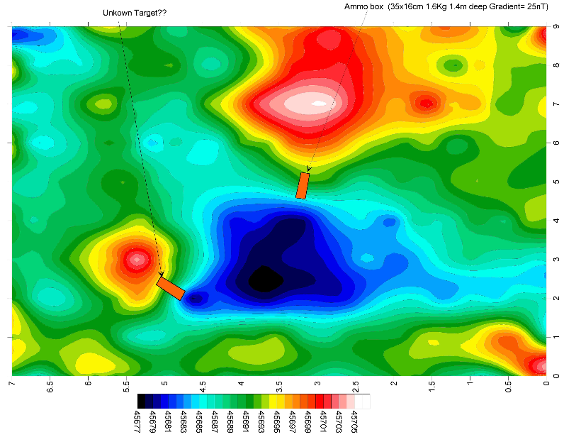
For the second test, an ammo box with a weight of 1.63kg was buried at a depth of 1.6m. The resultant dipole signal is greater than 50nT peak-to-trough. Also notice the dipole signature of an unknown target. Given the higher frequency (narrow width) of this target, one could interpret it as being at a depth shallower than 1.4m.
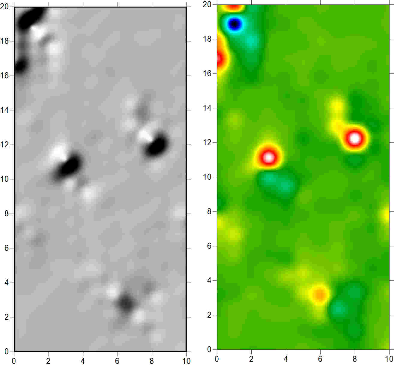
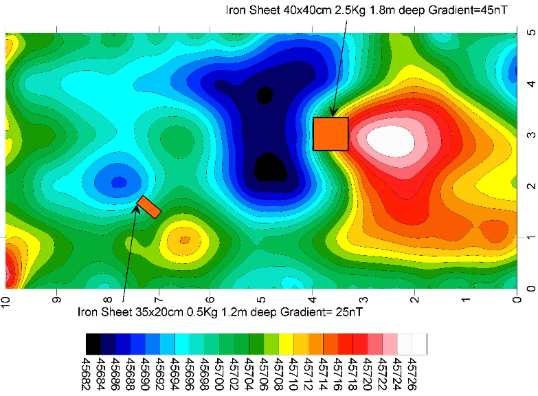
The third test shows two simple objects of different weights buried at two different depths in two different orientations. The bigger one generates a large field gradient of around 45 nT (this is the difference between the total field at the positive peak and the total field at the negative peak). The 0.5kg target is interesting as its greater than 20nT signal is obvious. So we conclude that even a half kg iron target is detectable at depths greater than 1.2m. All the color changes shown along the borders of the surveys have to be ignored; they are measurement and gridding artifacts. If the survey area had been much larger, these peaks would show like mountains in the middle of a flat desert.
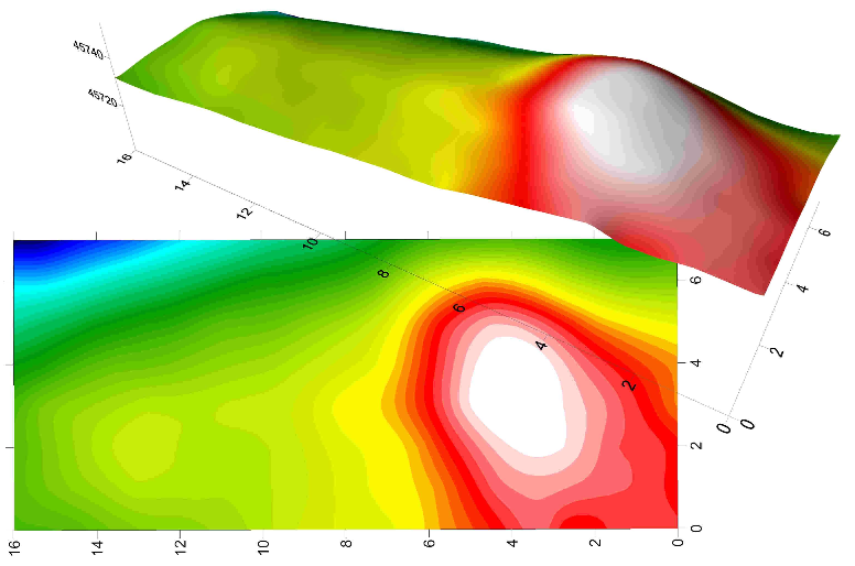
Test 4 is the most difficult to interpret as it shows a multiple target buried rather deep (almost 3 meters). Also, the survey area was rather small, just to enclose the target surface, for a reason of survey time and effort. During this survey, we can see that there were some surrounding disturbances (the red area in the S-E corner). This can be due to unknown buried material.
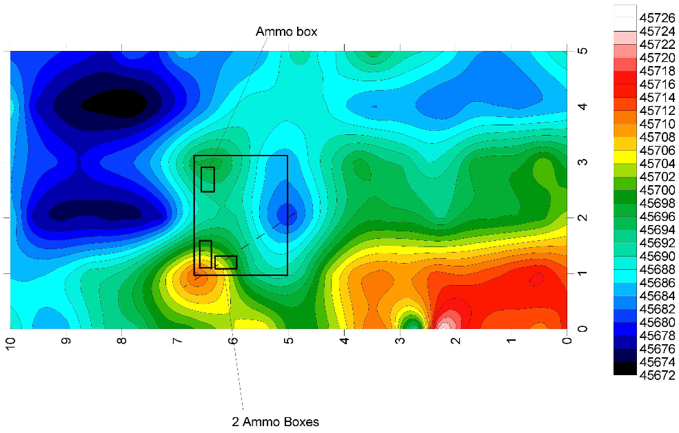
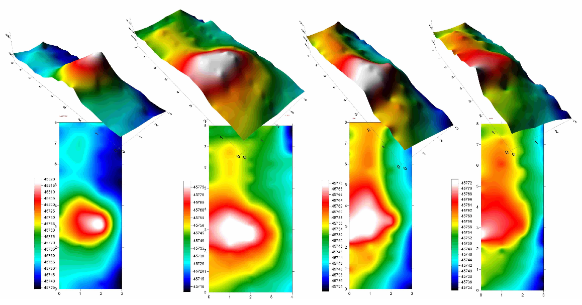
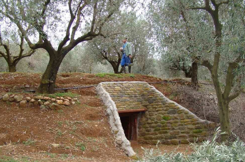 The final test that we present, is a depth test performed by one of our clients. A tunnel has be dug at a depth of 2.7m under a road and a bunch of empty ammunition boxes have been put in the tunnel. Survey grids were then made over this deep target and the results plotted in 2D and 3D. The rightmost plot is with 4 boxes, next is 7 boxes, next is 11 boxes and the last, leftmost plot has been made with 11 boxes elevated in the tunnel to reduce the depth to around 2m. Note that an (expensive) EMI sensor device (those so-called ‘deep target’, two-boxes types of detector) has been used for making surveys in the same conditions and this did not even detect the presence of the last 11 boxes.
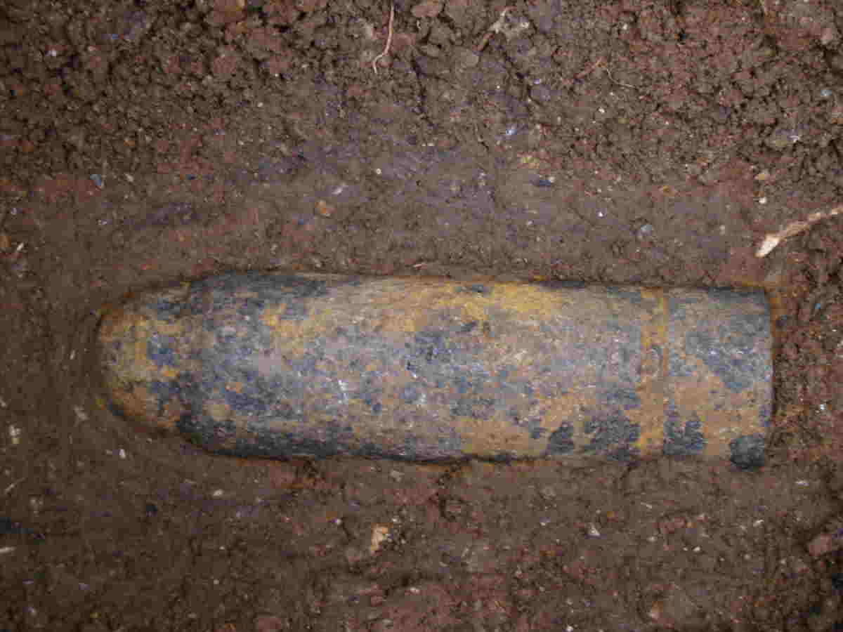
Real Target
This cannon shell has been located at more than 80cm deep.