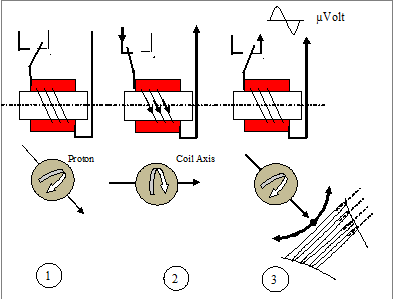
Normally, proton particles contained in fluids turn around their main axis but this axis also oscillates at a slower precession speed (a spinning top shows this very clearly) whose value uniquely depends on the value of the ambient magnetic field. In a normal status, the precession movement is not synchronized between protons and thus has a cancelling effect.
A sensor filled with a proton-rich fluid is placed in a coil at right angles to the ambient magnetic field and a strong current energizes the coil, creating a strong magnetic field – the so-called polarization field, which orients all the protons of the fluid in the same direction and stops their precession. When the polarization current is sharply ended, all the protons resume their normal precession but now, IN PHASE and thus, the accumulated action of all these very small magnets induces a VERY SMALL (at the µVolt RMS level) Audio Frequency Sine Wave signal in a signal pick-up coil (which could be the same as the polarization coil). This sine wave signal has a frequency depending ONLY on the TOTAL value of the local magnetic field vector and lasts a few seconds (the relaxation time) during which the precession of the protons still stays in phase. This frequency is called the ‘Larmor’ frequency. This voltage is amplified and its frequency precisely measured to determine the ambient field strength.
The exact relationship between ambient magnetic field (B in nT) and Larmor frequency (f) is the following:
B = f * 100,000 * 2 * PI / 26751.2 or B = f * 23.4875
f = B * 0,04256
For example, for an average ambient field of 50,000nT, f will then be 2.128 KHz
From the above relation, it is quite obvious that a difference of 1 Hz in frequency corresponds to a bit more than 23 nT. If a system should be built with a resolution of 1nT, then the Larmor frequency should be evaluated with at least an accuracy of 1 part in 50,000 or approximately, a precision of 0.04 Hz to have any chance to be successful. Moreover, depending on the proton-rich fluid that has been used in the sensor, the duration of this signal with a sufficient RMS amplitude will only be from 1 to 5 seconds as it exponentially decays. Thus, the frequency evaluation must be made as soon as possible after the polarization cut-off to get its maximum amplitude (and maximum SNR). However, this RMS voltage will not exceed a value in the order of 1µV. Its value will mostly depend on the fluid being used, on the polarization current and on the inductance of the signal pick-up coil.
There is a long list of proton-rich fluids that can be used in PPM sensors but, in practice, some liquids are usually rejected because they are potentially dangerous to manipulate. The most usual liquids being used by hobbyists are:
- Simple distilled or de-mineralized water (better boiled to remove dissolved oxygen (longer relaxation time) giving a comfortable relaxation time of 3 seconds but subject to freezing.
- Methyl, Ethyl Alcohol, Kerosene (lamp or stove oil), Diesel Fuel or charcoal lighter fluid with a shorter polarization and relaxation periods of 0.5 second but not subject to freezing
- Automotive windshield washer fluids
- Benzene with a longer relaxation time of 4 to 5 seconds but rather difficult to find by non-professionals.
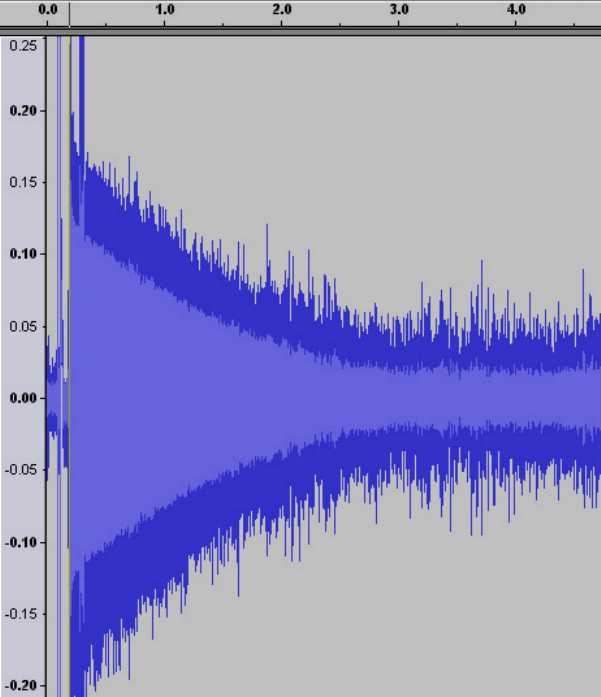
You can see here the exponential decay of the magnitude of a typical PPM signal generated after its polarization current has been cut off.
Listen to it here under:
This is its equivalent frequency spectrum (FFT) with its high and very narrow peak showing that it is a pure sine wave with some background noise.
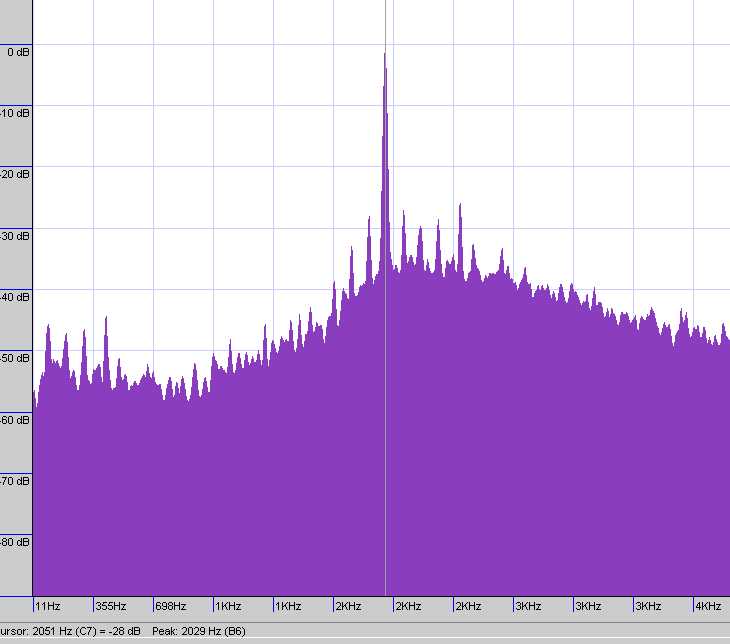
Its Signal-To-Noise Ratio (SNR) is around 35dB at 2KHz, this is not too good but, if we remove a good amount of this noise from the raw signal (with analogue or digital filtering) , we get this FFT result.
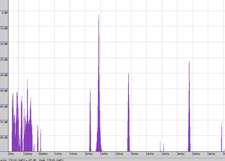
As you see, the Signal-To-Noise Ratio (SNR) jumped up to 90dB. Now, listen to it and hear the difference.
The magnitude of this signal was rather low but with a higher gain amplifier, this is what the digital filtering should give as result.
DIFFICULTIES OF THE MEASUREMENTS
The technical difficulties of such a device are filtering and amplification : one must be able to measure differences of 1 nT on a magnetic field of 50000 nT or measure frequency differences of 0.04 Hz .
This measure must be from a decaying AC signal which has only a peak-to-peak amplitude of few µV and must be read in a few hundreds of millisecond . That needs to be substantially amplified up to a hundred of mV and filtered to remove any “ambient noise” outside of the required precession frequencies before being converted to a digital value (with an ADC), analyzed and measured.
The required accuracy from a reasonably good magnetometer is then 0.002 % . As a comparison, any standard measurement device has generally an accuracy of 1% .
TUNING of a PPM
For high sensitivity and accuracy operation, the device must be tuned to the local frequency. This is the same type of operation being done with a radio on a desired frequency. A tuned sensor gives a signal (sine wave) of higher peak-to-peak magnitude as the tuning has an amplification effect on signals whose frequency is the center (resonant) frequency. This is done in each region of exploration before a series of measurements.
The tuning must of course be done in a place free from any electromagnetic disturbance (vehicle, concrete re-bar , … )
The device gets an amplification gain from the resonant circuit RLC ( resistance – inductance – capacitance) consisting of the sensor coils (L + R ) , the cable ( R ) and a number of capacitors in parallel ( C ) contained in the control box.
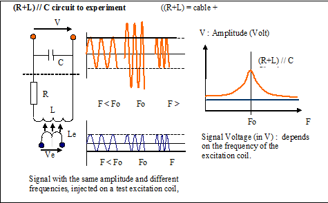
In this type of amplification , the amplification gain is not constant , it depends on the frequency of the signal to be amplified . There is a peak amplification gain for a given frequency , depending on the values of the RLC . This frequency is the resonant frequency . The tuning will find the value of the capacitance C to maximize the amplification at the resonance of the frequency of the measured local magnetic field. This maximum amplification will allow the further frequency measurements to work in good conditions
The tuning operation is done in two steps , the measurement phase and the adjustment .phase.
During measurement, the capacitance of the RLC circuit is switched off , only the sensor and the cable are connected to the device. The lack of capacitance has as consequence that no specific frequency will be enhanced by a resonance .
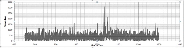
One then powers the sensor, then, its power supply is cut off and the received signal is captured, stored and analyzed with an FFT algorithm. We make a frequency analysis of this FFT result by scanning the possible frequencies of the geomagnetic field between 1300Hz and 2600 Hz (30000nT to 60000nT ) . It is the frequency that has the highest level in mV that is selected to be used in the second phase for that region.
Spectrum measured by the PPM( by Excel )
The second step , the setting is to tune in to that frequency , so that the amplification is maximal for this value. The readings will be very accurate.
In practice, we calculate the capacitance given the inductance of the resonant circuit and the frequency measured by the FFT process, then we test all capacitances around this first one by measuring each time the ambient magnetic field value and stepping up and down a few nF at a time . The one giving the best amplification in mV of signal and the lowest standard deviation is the one to record.
Once this setting is made , the surveys can be made in that same region with the optimum precision.
These operations are fully automated on the PPM , they only last about 1 minute .